LIS Public Testcase Walkthrough

Table of Contents

Introduction
Setup
Step 1: LSM Parameter Processing Run (LDT)
Step 2: LSM "Open-loop" (OL) Experiment (LIS)
Step 3: Ensemble Restart File Generation (LDT)
Step 4: Generate LSM OL Cumulative Density Function-based Files (LDT)
Step 5: Generate Observations CDF-based Files (LDT)
Step 6: LSM Data Assimilation (DA) Experiment (LIS)
Step 7: Comparison of OL and DA Experiments (LVT)

Introduction

The Land Information System framework (LISF) public testcases described in this document provide users a suite of step-by-step experiments to learn how to run and test the LISF code. These experiments include a full end-to-end walkthrough of all three (3) components of the LISF; (1) the Land Data Toolkit (LDT), (2) the Land Information System (LIS), and (3) the Land Verification Toolkit (LVT). These testcases demonstrate how to use LDT to generate model parameter and assimilation-based input files, how to use LIS to run the Noah land surface model (LSM) for a sample "open-loop" (or baseline) experiment and a data assimilation (DA) experiment, and how to use LVT to compare output from the sample experiments. The testcases were created to demonstrate the use of LISF, however, the files provided could be expanded to support research-related model runs.

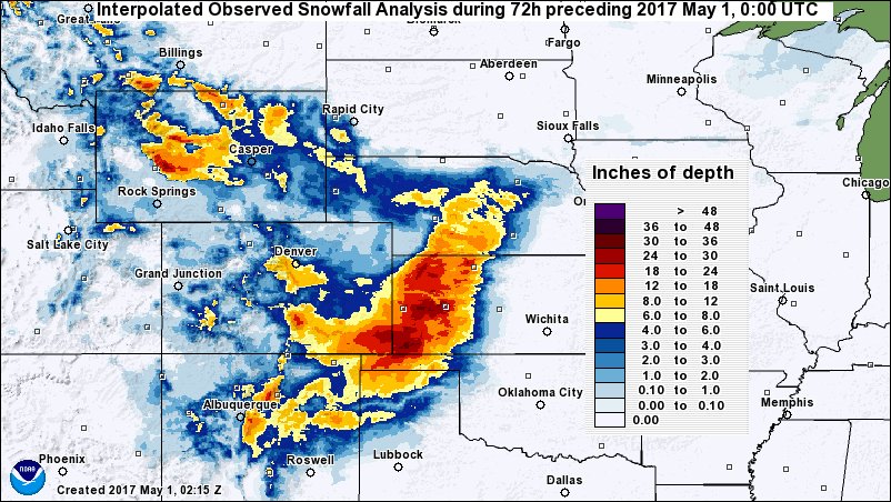
The Testcase Event: Snow Blankets the Southern Great Plains

In late April of 2017, a major snow storm event occurred across the Southern Great Plains (SGP) and Rocky Mountains, an area spanning Colorado, Texas, Oklahoma, and southern Kansas. This storm event will be the focus of these testcases.

(Image source, Data source)

Setup

If you have not set up your computing environment to compile and run the LISF code, review the official documentation.

Users on NASA’s NCCS Discover HPC system should review Quick Start Guide for NCCS Discover Users in our docs.

Create a working directory

To begin, create and step into a working directory that you will use throughout the testcases. This directory will be referred to as $WORKING_DIR from this point forward. In the following example, we create a working directory called lis-public-testcases:

% mkdir lis-public-testcases
% cd lis-public-testcases

Clone the LISF Repository

From inside your $WORKING_DIR, clone the public support branch of the LISF repository:

% git clone -b support/lisf-public-7.4 github:NASA-LIS/LISF.git
% cd LISF

The support/lisf-public-7.4 branch is known to be compatible with the testcase files. The master branch may contain changes to the LISF source code that break compatibility with the testcase files. We therefore recommend using the support branch while working through these testcases.

Configure and Compile the LISF Components

For information about configuration settings and detailed compilation instructions, see the LISF Users' Guides. In general, the compilation process for each component is as follows:

As you run these testcases, you will have the opportunity to compare your output to TARGET_OUTPUT files or "solutions". The TARGET_OUTPUT files were created by running ldt, lis, and lvt compiled with default compile configuration settings. For this walkthrough, it is recommended that you also use default compiler configuration settings.

% cd ldt
% ./configure
> # Select compile configuration settings (Default settings recommended.)
% ./compile
> # Compilation output...
% mv LDT ../../            # move executable up into $WORKING_DIR
% cd ..                    # change directories back into LISF

Repeat the above process in the lis/ and lvt/ directories to generate the LIS and LVT executables.

Change directories back into your $WORKING_DIR which should now contain three executable files: LDT, LIS, LVT.

If you ever wish to generate new executable files, cd into /LISF/l??/make and run gmake realclean. This will clear all dependency files and allow you to cleanly define new compile configuration settings and recompile.

Step 1: LSM Parameter Processing Run (LDT)

Overview

In this step you will learn how to run LDT to perform parameter processing for the Noah-3.6 land surface model (LSM) and generate a Noah-3.6 parameter input file which will be used by LIS and LVT in later steps.

Steps to Running LDT

Gather input data needed by LDT
Modify ldt.config file to define runtime configuration settings
Run the LDT executable
Examine output

These testcases were designed to be run in sequential order and later steps require the output generated by earlier steps.

Download Input and Target Files

The tar file for this step is approximately 350MB compressed and 4.2GB unpacked. Ensure that you have enough storage available before downloading testcase files.

The tar files used in this walkthrough are available on the LIS Testcase website. From within your $WORKING_DIR, download and unpack the compressed tar file containing the inputs and target outputs for Step 1:

% curl -O https://portal.nccs.nasa.gov/lisdata_pub/Tutorials/Web_Version/testcase1_ldt_parms_2023.tar.gz
% tar -xzf testcase1_ldt_parms_2023.tar.gz -C .

In addition to the LISF/ directory and the three executables, your $WORKING_DIR should now contain the following directory and files:

INPUT/

A directory that will hold parameter and input files needed throughout the testcases

ldt.config.noah36_params

The runtime configuration file read by LDT in this step

target_lis_input.nldas.noah36.d01.nc

The "target" NetCDF file generated by LDT in this step

target_log/

A directory containing the "target" mask-parameter log and the "target" ldt diagnostic file generated by LDT in this step

Files and directories beginning with target are provided to compare with the output of your run.

The LDT Configuration File

The LDT configuration file contains input settings used by LDT at run-time to generate input files for LIS. The configuration options are described in depth in the LDT Users' Guide.

Before continuing, review the contents of the LDT configuration file for our LDT-based Noah.3.6 parameter testcase by printing the file contents to the terminal with cat or opening the file with a text editor such as vim or emacs. Key elements of the file are highlighted below:

#Overall driver options
LDT running mode:                   "LSM parameter processing"
Processed LSM parameter filename:   ./lis_input.nldas.noah36.d01.nc (1)
LIS number of nests:                1
Number of surface model types:      2
Surface model types:                "LSM" "Openwater"
Land surface model:                 "Noah.3.6" (2)
...
LDT diagnostic file:                ldtlog (3)
LDT output directory:               OUTPUT (4)
Undefined value:                    -9999.0
...
#LIS domain (5)
Map projection of the LIS domain:  latlon
Run domain lower left lat:         34.375
Run domain lower left lon:         -102.875
Run domain upper right lat:        39.625
Run domain upper right lon:        -96.125
Run domain resolution (dx):        0.25
Run domain resolution (dy):        0.25

# Parameters
Landcover data source:             MODIS_Native (6)
Landcover classification:          IGBPNCEP
Landcover file:                    ./INPUT/LS_PARAMETERS/noah_2dparms/igbp.bin (6)
Landcover spatial transform:       tile
...

1	The name of the NetCDF-formatted parameter file to be generated which will be used by LIS
2	The LSM to run (e.g., Noah.3.6)
3	The name of the diagnostic log file
4	The directory where LDT output will be placed
5	The grid projection, domain extents, and spatial resolution to be used by LIS (and LVT)
6	Data source settings and paths (e.g., landcover datasets, elevation datasets) and additional features of interest (e.g., irrigation settings)

LISF configuration files use relative paths to describe file locations. Keep this in mind if you encounter any "file not found" errors.

Noah Land Surface Model Parameters

As you may have noticed, these testcases utilize NOAA/NCAR’s Noah LSM, v3.6. The input parameters selected in ldt.config.noah36_params include:

Parameter	Dataset
Landcover	MODIS-based IGBP landcover map (~ 1 km, NOAA)
Soil texture	FAO+STATSGOv1 combined soil texture map (~ 1 km, NOAA)
Greenness fraction	AVHRR-based monthly climatology (1.0 deg, NOAA)
Snow-free albedo	Monthly climatology dataset (1.0 deg, NOAA)
Maximum snow albedo	MODIS-based maximum snow albedo (0.05 deg; Mike Barlage, NCAR)
Bottom of soil column temperature	ISLSCP-1 climatology dataset (1.0 deg)

Parameter

Dataset

Landcover

MODIS-based IGBP landcover map (~ 1 km, NOAA)

Soil texture

FAO+STATSGOv1 combined soil texture map (~ 1 km, NOAA)

Greenness fraction

AVHRR-based monthly climatology (1.0 deg, NOAA)

Snow-free albedo

Monthly climatology dataset (1.0 deg, NOAA)

Maximum snow albedo

MODIS-based maximum snow albedo (0.05 deg; Mike Barlage, NCAR)

Bottom of soil column temperature

ISLSCP-1 climatology dataset (1.0 deg)

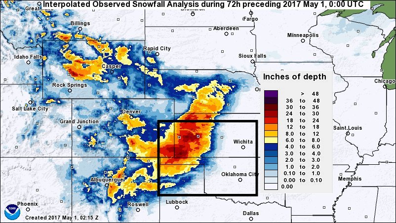
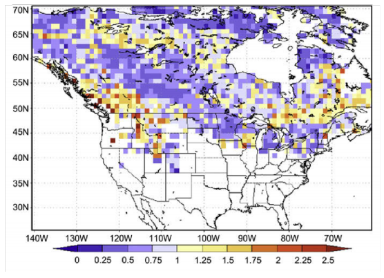
Testcase Domain

The spatial domain defined in the LDT configuration file will be placed in lis_input.nldas.noah36.d01.nc, the NetCDF-formatted parameter file generated by LDT which LIS will read in automatically at run-time. For these testcases we will be using the domain depicted by the black box on this map:

Testcase domain

Run LDT - The Parameter Processing Step

You’re now ready to run LDT:

Copy your compiled LDT executable into $WORKING_DIR/
Run the LDT executable using the provided ldt.config.noah36_params file:

% ./LDT ldt.config.noah36_params

The run should take a few minutes to complete. If the run aborts, troubleshoot the issue by reviewing any errors printed to the terminal and by viewing the contents of ldtlog.0000. If no errors print to the terminal, verify that the run completed successfully by checking for the following confirmation at the end of the ldtlog.0000.

If the terminal reports the error "./LDT: symbol lookup error:", this may be due extraneous modules loaded into your environement that do not allow lis to run properly. View your modules using the command module list. If extraneous modules are loaded, run module purge to clear your environment and then module load [lisf module file] to load an environment suitable to running LISF. See the "discover_quick_start" document in the LISF Users' Guides for more information.

% tail ldtlog.0000
...
 --------------------------------
  Finished LDT run
 --------------------------------

ldt, lis, and lvt can also be run by submitting batch jobs using SLURM (Simple Linux Utility for Resource Management). If you are running this tutorial on Discover, you can download example batch scripts for all steps from the LIS Testcase website using the following command:

% curl -O https://portal.nccs.nasa.gov/lisdata_pub/Tutorials/Web_Version/testcase_batch_scripts.tar.gz
% tar -xzf testcase_batch_scripts.tar.gz -C .

The batch scripts (step*.job) will unpack into the appropriate directories. To submit a job to discover using a batch script, use the command sbatch [BATCH SCRIPT] from the same directory as the job you wish to run. The command squeue -u [YOUR USER ID] will provide updates on your job. If the job crashes, troubleshoot using any slurm.out files.

See the NCCS Discover Jobs Users' Guide for more information.

LDT Output Files

The following files are typically generated by an LDT parameter processing run:

lis_input.nldas.noah36.d01.nc

The NetCDF-formatted model parameter file which LIS reads at runtime. d01 refers to the indexed domain, typically used as "nests" for NASA-Unified WRF simulations.

ldtlog.0000

The output diagnostic file that provides runtime messages, including warnings and error messages. This file is useful for verifying successful run completion and troubleshooting unsuccessful runs.

MaskParamFill.log

This diagnostic file informs of any disagreements between an LSM-based parameter and the landmask, and whether any parameter gridcells were "filled" to agree with the landmask.

The output filenames for lis_input.nldas.noah36.d01.nc and ldtlog.0000 can be defined in the ldt.config file, but the filename of MaskParamFill.log cannot be modified.

The LIS Parameter File

The contents of the LIS parameter input file produced by LDT can be examined visually using a command-line program such as ncview or a desktop application like NASA’s Panoply. For this walkthrough we will be using ncview. If needed, add ncview to your environment by running, module load ncview.

Open the LIS input file using ncview:

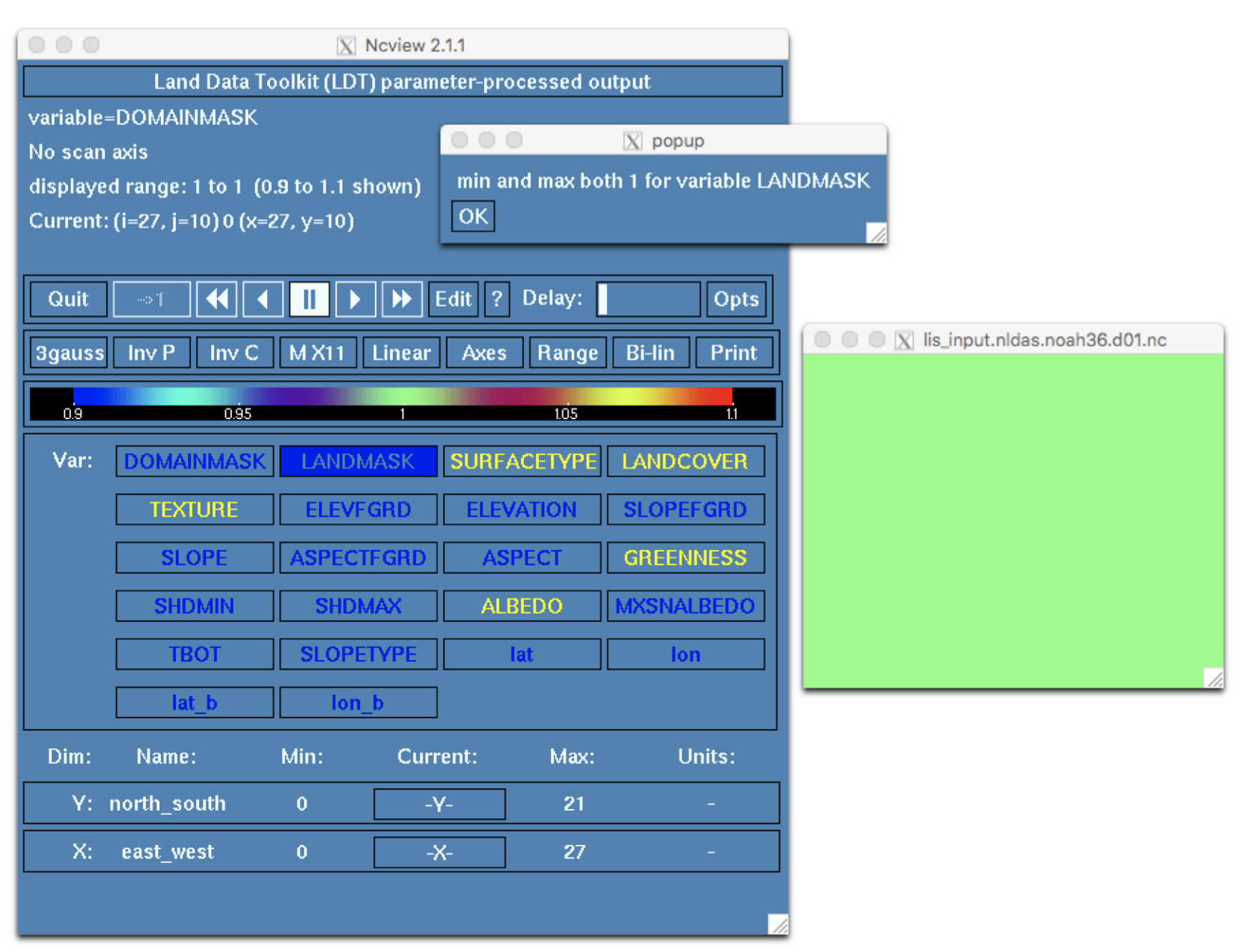
% ncview lis_input.nldas.noah36.d01.nc

In the ncview window that opens, click on the widget labeled DOMAINMASK. A second window will open containing a map of the mask. The domain we are using is a simple rectangle so, as expected, all values are equal to 1.

Click on the widget labeled LANDMASK. Again, the values are all equal to 1. This indicates that all grid cells within the domain are treated as land and, as a result, the input file should not contain any undefined values (e.g., -9999).

LANDMASK dataset

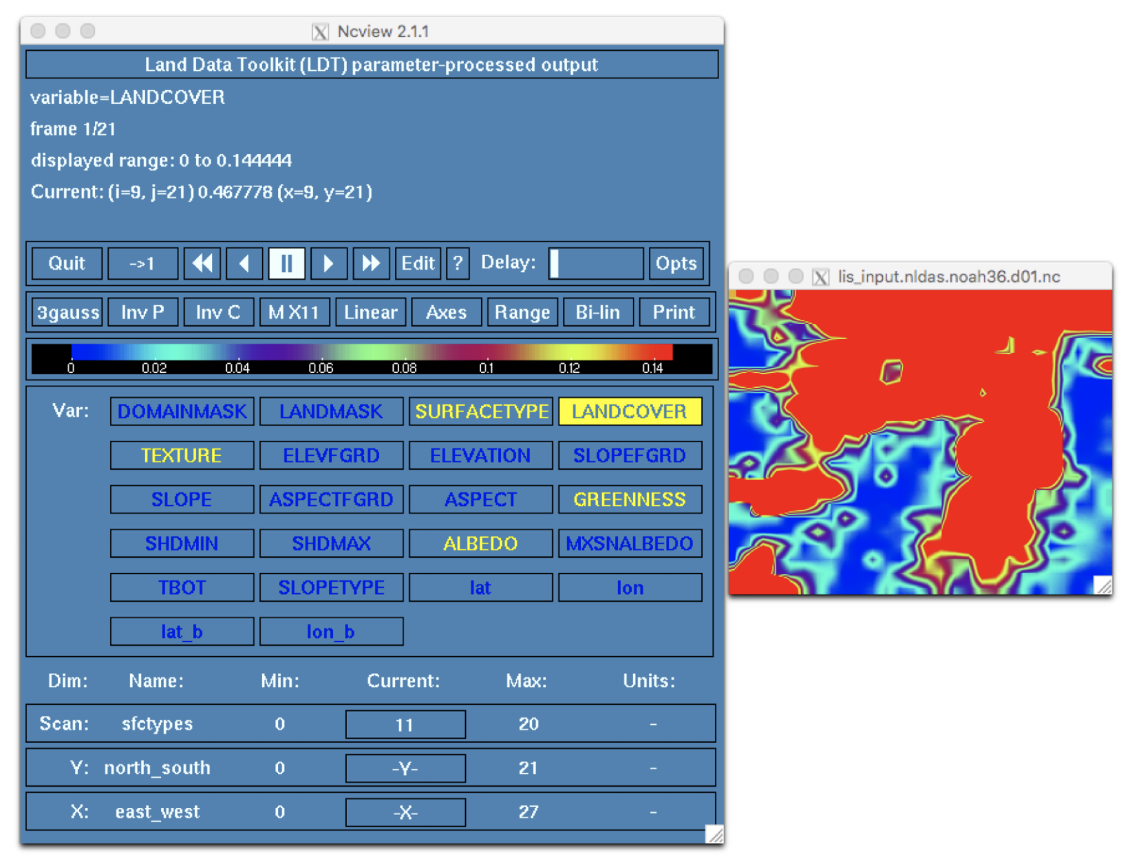
Click on the LANDCOVER widget to view the landcover variable. In the bottom third of the ncview window, click on the widget below the label Current to cycle through the 20 different IGBP landcover and land use classes. In the screenshot below the Crop class is selected (the classes are zero-indexed in ncview; add 1 to index to convert to IGBP class).

The Crop class of the LANDCOVER dataset

Click on the TEXTURE widget to view the soil texture dataset. Click on the widget below the label Current. This is the FAO+STATSGO soil texture map, aggregated using the tile option for the Soil texture spatial transform: setting in ldt.config. The map shows the fraction, or frequencies, of each soil type within each 0.25° degree grid cell of our domain.

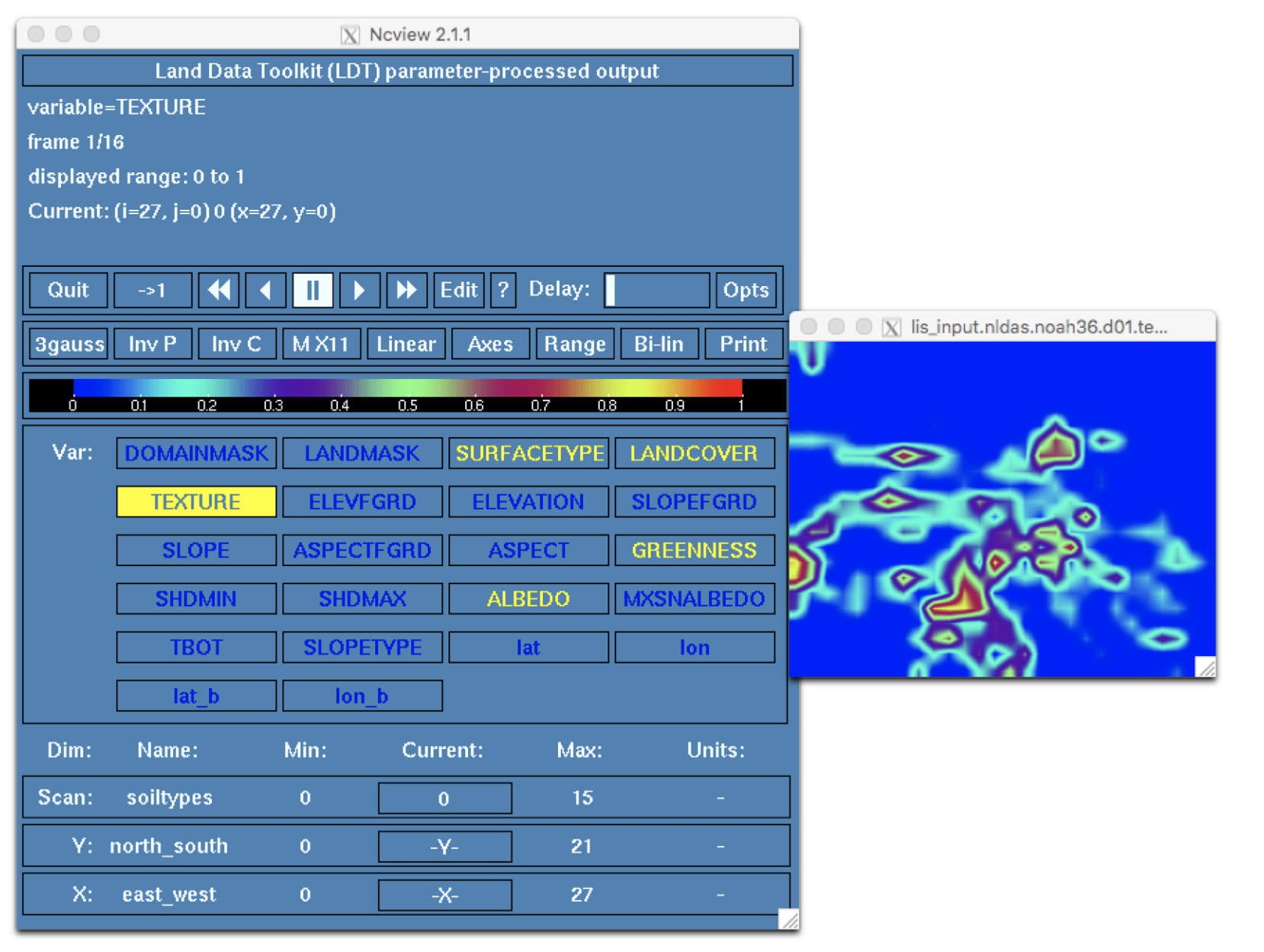
Soil texture, tile-based aggregation

LDT provides several other options for grid cell aggregation including none, mode, and neighbor. What would the output look like if we were to rerun LDT after switching from tile to mode? Open ldt.config.noah36_params in a text editor and change the Soil texture spatial transform option from tile to mode as below:

...
Soil texture spatial transform: mode
...

Rerun LDT:

% ./LDT ldt.config.noah36_params

Check the end of ldtlog.0000 to verify LDT ran successfully. Again, open the LIS input file using ncview and click on the TEXTURE widget.

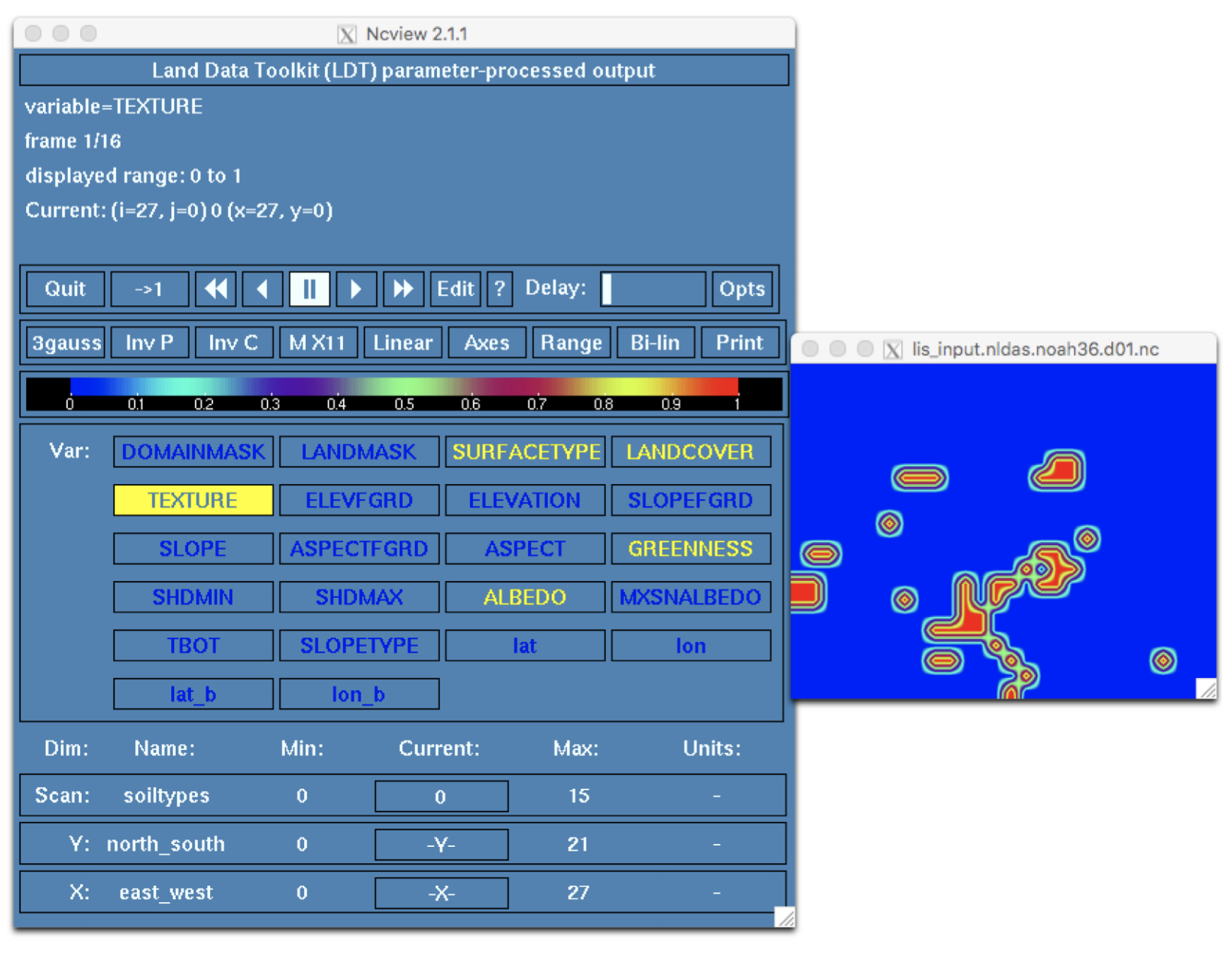
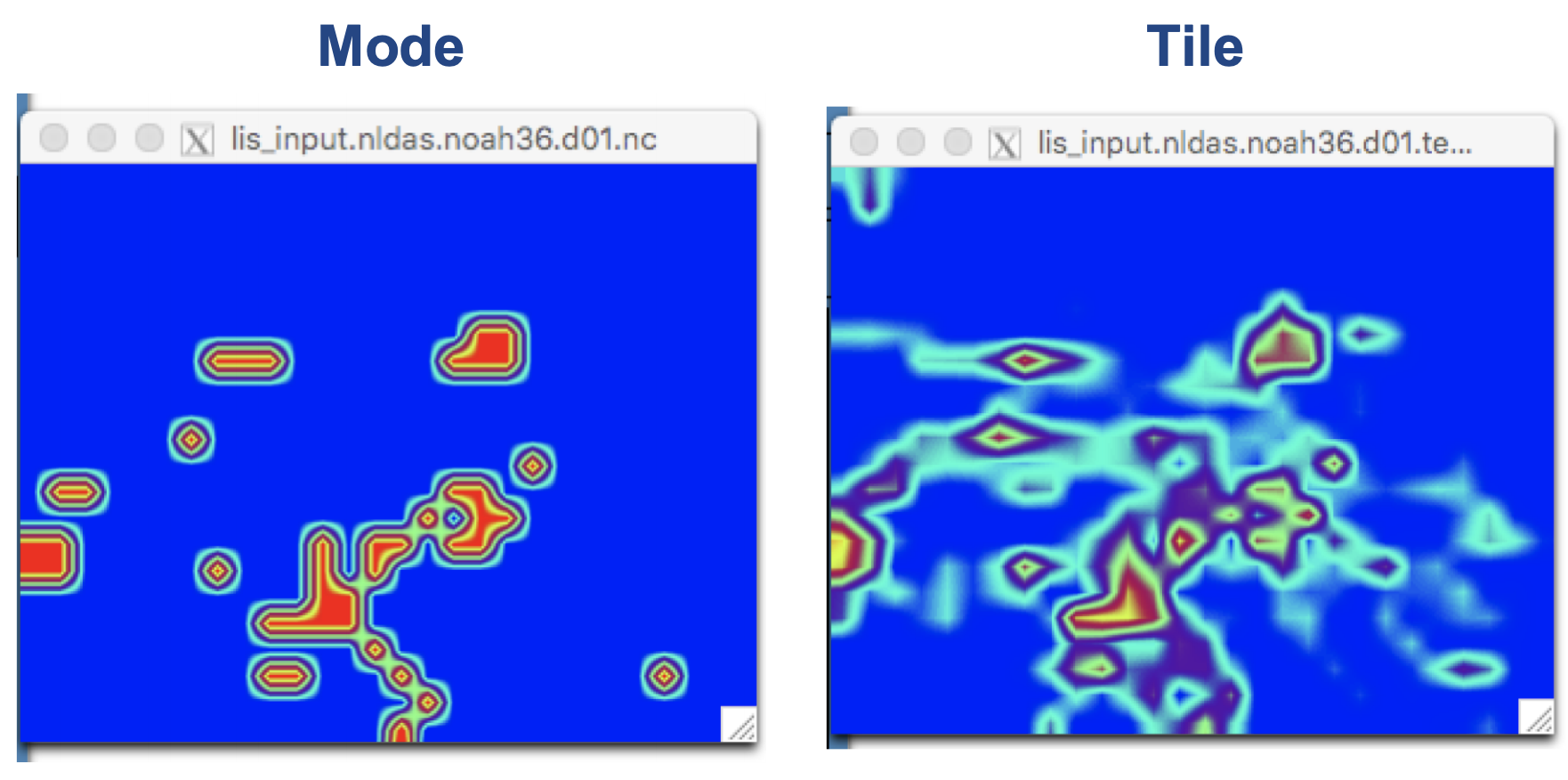
Each soil type now shows a total value of 1 within each 0.25 degree grid cell of our domain. Why? The mode option selects the dominant soil type for each grid cell.

For comparison:

Dominant vs. fractional soil type

Another program called ncdump can be used to directly view the datasets contained in NetCDF files. For example, the -h flag can be used to print the dimensions, variable names, and attributes of the file to the terminal:

% ncdump -h lis_input.nldas.noah36.d01.nc
netcdf lis_input.nldas.noah36.d01 {
dimensions:
    east_west = 28 ;
    north_south = 22 ;
    east_west_b = 32 ;
    north_south_b = 26 ;
    month = 12 ;
    time = 1 ;
    sfctypes = 21 ;          # Note: 21 includes “openwater” surface type
    soiltypes = 16 ;
    elevbins = 1 ;
    slopebins = 1 ;
    aspectbins = 1 ;
variables:
    float time(time) ;
    float DOMAINMASK(north_south, east_west) ;
          DOMAINMASK:standard_name = "DOMAINMASK" ;
          DOMAINMASK:units = "" ;
          DOMAINMASK:scale_factor = 1.f ;
          DOMAINMASK:add_offset = 0.f ;
          DOMAINMASK:missing_value = -9999.f;
          DOMAINMASK:vmin = 0.f ;
          DOMAINMASK:vmax = 0.f ;
          DOMAINMASK:num_bins = 1 ;
global attributes:
    :MAP_PROJECTION = "EQUIDISTANT CYLINDRICAL" ;
    :SOUTH_WEST_CORNER_LAT = 34.375f ;
    :SOUTH_WEST_CORNER_LON = -102.875f ;
    :DX = 0.25f ;
    :DY = 0.25f ;
    :INC_WATER_PTS = "true" ;
    :LANDCOVER_SCHEME = "IGBPNCEP" ;
    :BARESOILCLASS = 16 ;
    :URBANCLASS = 13 ;
    :SNOWCLASS = 15 ;
    :WATERCLASS = 17 ;
    :WETLANDCLASS = 11 ;
    :GLACIERCLASS = 15 ;
    :NUMVEGTYPES = 17 ;
    :LANDMASK_SOURCE = "MODIS_Native" ;
    :SFCMODELS = "Noah.3.6+Openwater" ;
    :SOILTEXT_SCHEME = "STATSGO" ;
    :GREENNESS_DATA_INTERVAL = "monthly" ;
    :ALBEDO_DATA_INTERVAL = "monthly" ;

Compare the Output

To further confirm that LDT ran successfully, you can compare your output with the "target" output included with the input files you downloaded earlier (files or directories beginning with target_). For example, use nccmp to compare your lis_input.nldas.noah36.d01.nc with target_lis_input.nldas.noah36.d01.nc:

% nccmp -dfs lis_input.nldas.noah36.d01.nc target_lis_input.nldas.noah36.d01.nc

Where the flags d, f, and s enable the following options:

d: compare data
f: force comparison to continue after differences found
s: report identical files to terminal (by default nccmp runs silently if files are identical)

The nccmp command will be used in future steps. Going forward, some files may not be identical, but any differences reported should be small. Also note: in this step, the target lis input file was generated using Soil texture spatial transform: mode

Wrap-up

The LDT parameter processing run generates input parameters and files that LIS requires. Your $WORKING_DIR should now contain all the files needed to continue on to the next step.

Step 2: LSM "Open-loop" (OL) Experiment (LIS)

Overview

In this step you will learn how to run LIS with the Noah-3.6 LSM for an "open-loop" case. This testcase uses the files generated by LDT in Step 1.

Steps to Running LIS

Download input data (e.g., meteorolgical forcing, observations)
Modify the lis.config file to select runtime options
Run the LIS executable
Examine output

Download Input and Target Files

The tar file for this step is approximately 65MB compressed and 343MB unpacked. Ensure that you have enough storage available before downloading testcase files.

% curl -O https://portal.nccs.nasa.gov/lisdata_pub/Tutorials/Web_Version/testcase2_lis_ol_2023.tar.gz
% tar -xzf testcase2_lis_ol_2023.tar.gz -C .

The following files and directories were added to your common working directory, $WORKING_DIR:

INPUT/wget_gesdisc_nldas2.sh

A script to download NLDAS2 forcing data

INPUT/NOAH36_OUTPUT_LIST.TBL

Model output specification

INPUT/forcing_variables.txt

Forcing variable specification

INPUT/LS_PARAMETERS

Model parameter specification

lis.config_noah36_ol

The runtime configuration file that will be read by LIS

target_log/lislog_ol.0000

The "target" log file that should be produced by LIS in this step

target_OL_OUTPUT/

A directory containing containing the "target" open-loop (OL) output files that should be generated by LIS in this step

target_ol.xdf

GrADS descriptor file for visualizing outputs

Download the Meteorological Forcing Dataset

This testcase is set up to use the North American Data Assimilation System, version 2 (NLDAS-2) meteorological forcing dataset available from NASA GES DISC. A script has been provided in the input files that uses wget to download these data.

Users on NASA’s NCCS Discover HPC system do not need to download the data as described below. Instead, change directories into INPUT/ and create a symbolic link to a local copy:

% ln -s /discover/nobackup/projects/lis/MET_FORCING/NLDAS2.FORCING NLDAS2.FORCING

Jump to the next step.

Before running the download script:

If needed, install wget
Create a NASA Earthdata account if you do not already have one
Follow steps 1-3 in these instructions to save your NASA Earthdata login credentials locally

When you are ready to run the script, change directories into INPUT/ and run the following command:

% sh wget_gesdisc_nldas2.sh

The script will download NLDAS-2 forcing data for the entire year of 2017 into a directory named NLDAS2.FORCING/. If the script completes without any errors, change up one directory back to your $WORKING_DIR. If any errors are thrown, attempt to resolve them.

The LIS Configuration File

The main LIS configuration file (lis.config_noah36_ol) is where runtime options and filepaths used during the run are defined. These include:

The LSM of interest (e.g., Noah.3.6)
The name of the NetCDF-parameter file created by LDT in the previous step (e.g., lis_input.nldas.noah36.d01.nc)
The name of the LIS diagnostic file (e.g., lislog)
The date and time inputs, model options, parallel domain entries, etc.
Meteorological forcing dataset(s) selected; also some downscaling features
Data assimilation entries, and other features, such as irrigation or runoff routing

Open the LIS configuration file in a text editor to view these settings and more.

You may notice that the grid domain is not contained in this file. The grid domain that was defined in the ldt.config file is now contained in the NetCDF-formatted parameter file (lis_input.nldas.noah36.d01.nc) and this information will be read by LIS at runtime.

Run LIS - The "Open-Loop" (OL) Step

You are now ready to run LIS.

In your $WORKING_DIR, execute the following command:

% ./LIS -f lis.config_noah36_ol

LIS can also be run in parallel. The examples in this walkthrough, however, demonstrate how to run LIS on a single processor. See Chapter 6 in the LIS Users' Guide for instructions for running LIS in parallel.

With a single processor the run should take approximately 20 minutes to complete. If the run fails, diagnose the issue by reviewing any errors that have printed to the terminal and by viewing the contents of lislog files (located in the log directory as defined by line 42 of lis.config_noah36_ol). If no errors appear and the run appears to have completed successfully, examine the end of any lislog files present to check for a confirmation message:

% tail lislog.0000
 [INFO] LIS cycle completed
[INFO] LIS cycle time: 01/01/2018 00:00:00
 [INFO] getting file2a..
 ./INPUT/NLDAS2.FORCING/2018/001/NLDAS_FORA0125_H.A20180101.0100.002.grb
 [ERR] Could not find file:
 ./INPUT/NLDAS2.FORCING/2018/001/NLDAS_FORA0125_H.A20180101.0100.002.grb
 [INFO] Noah-3.6 archive restart written:
 ./OL_OUTPUT/SURFACEMODEL/201801/LIS_RST_NOAH36_201801010000.d01.nc

  LIS Run completed.

Use ls to view the files and directories created by LIS.

LIS Output Files

The output files created by LIS were placed into a new directory called OL_OUTPUT. Within this directory is another directory called SURFACEMODEL which contains subdirectories following the naming convention YYYYMM:

YYYY 4-digit year
MM 2-digit month

Within each of those subdirectories are NetCDF-formatted LIS output files that contain the Noah-3.6 output variables defined in NOAH36_OUTPUT_LIST.TBL (e.g., soil moisture, runoff, evapotranspiration). Use any visualization package you are comfortable with to view the files (e.g., Matlab, GrADS, ncview). For GrADS users, descriptor files are provided with the input data.

Wrap-up

You have now generated your LIS Noah-3.6 model run for the open-loop case. Use diff and nccmp to compare the output files you generated with the "target" versions found in target_OL_OUTPUT/. As in Step 1, the files you generated in this step will be used in later steps.

Step 3: Ensemble Restart File Generation (LDT)

Overview

In Step 1, you used LDT to perform parameter processing for the Noah-3.6 land surface model (LSM) to generate a Noah-3.6 parameter input file to be used by LIS (and LVT). In addition to parameter processing, LDT can be used to upscale and downscale ensembles.

Upscale: generate a multi-member ensemble restart file from a single-member restart file

Downscale: generate a single-member ensemble restart file from a multi-member restart file

In this step you will learn how to use LDT to expand a single-member restart file generated by the LIS open-loop (OL) case in Step 2 into a restart file that contains an ensemble of size N (user specified). The ensemble restart file generated in this step will be used in Step 6 to initialize the LIS data assimilation (DA) run.

Restart files contain all of the initial condition information necessary to restart from a previous simulation.

— http://www.cesm.ucar.edu/models/ccsm2.0/csim/UsersGuide/ice_usrdoc/node21.html

Download Input and Target Files

The tar file for this step is approximately 97KB compressed and 100KB unpacked. Ensure that you have enough storage available before downloading testcase files.

% curl -O https://portal.nccs.nasa.gov/lisdata_pub/Tutorials/Web_Version/testcase3_ldt_ensrst_2023.tar.gz
% tar -xzf testcase3_ldt_ensrst_2023.tar.gz -C .

The following files and directories were added to your common working directory, $WORKING_DIR:

DA_ensrst/

A directory containing the files below

ldt.config

The LDT config file for this step

target_ldtlog.0000

The target LDT log file

target_LIS_EnRST_NOAH36_201801010000.d01.nc

The target LDT-generated ensemble restart file ("EnRST") to start the Noah LSM DA run in Step 6

The LDT Configuration File

Review the contents of DA_ensrst/ldt.config to view the configuration settings used for this step:

LDT running mode:                               "Ensemble restart processing"
Processed LSM parameter filename:               ./lis_input.nldas.noah36.d01.nc
...
LIS restart source:                             "LSM"
Ensemble restart generation mode:               "upscale" (1)
Input restart filename:                         ../OL_OUTPUT/SURFACEMODEL/201801/LIS_RST_NOAH36_201801010000.d01.nc
Number of ensembles per tile (input restart):   1 (2)
Number of ensembles per tile (output restart):  12 (3)

1	This entry tells LDT how to process the ensemble file
2	Size of input ensemble restart file, in this case a single instance of model states
3	Size of upscaled multi-member ensemble restart file, in this case 12 members

In this walkthrough we are using the Noah.3.6 LSM, but these settings can be used to upscale/downscale routing models as well. For example:

LIS restart source:                             "Routing"
Ensemble restart generation mode:               "upscale"
Input restart filename:                         ./LIS_RST_HYMAP_router_201801010000.d01.bin
Output restart filename:                        ./ensrst.bin
Number of ensembles per tile (input restart):   1
Number of ensembles per tile (output restart):  12

Run LDT - Generate Ensemble Restart File

You’re now ready to run LDT:

Copy your compiled LDT executable into $WORKING_DIR/DA_ensrst
Run the LDT executable using the provided ldt.config file:

% ./LDT ldt.config

% tail ldtlog.0000
...
 --------------------------------
  Finished LDT run
 --------------------------------

LDT Output Files

During this run, LDT produced one output file named LIS_EnRST_NOAH36_201801010000.d01.nc and placed it into the $WORKING_DIR/DA_ensrst directory.

Use ncview, Panoply, Matlab or any other viewing package that supports NetCDF files. Compare what you see with the target version of this output file, also located in $WORKING_DIR/DA_ensrst. Additionally, you can use nccmp to directly compare the contents of the file created by your LDT run and the target. If there are differences between your file and the target file, you can use ncdiff to create a new NetCDF file to visualize the differences.

Step 4: Generate LSM OL Cumulative Density Function-based Files (LDT)

Overview

In the previous step you used LDT used to expand a single-member ensemble restart file into a multi-member restart file containing 12 ensemble members. In this step you will use LDT again to generate files that support scaling and bias-correction between the model open-loop states and satellite observations that will be assimilated in Step 6. LDT supports the generation of domain and statistical moment inputs for estimated cumulative distribution functions (CDFs), which can be used when performing the scaling necessary to assimilate certain observations in LIS. The model-based CDF files generated in this step, and those generated in Step 5 for the satellite observations, will be incorporated in the data assimilation run demonstrated in Step 6.

CDF-based scaling is used to match the CDF of a given observation to that of the model.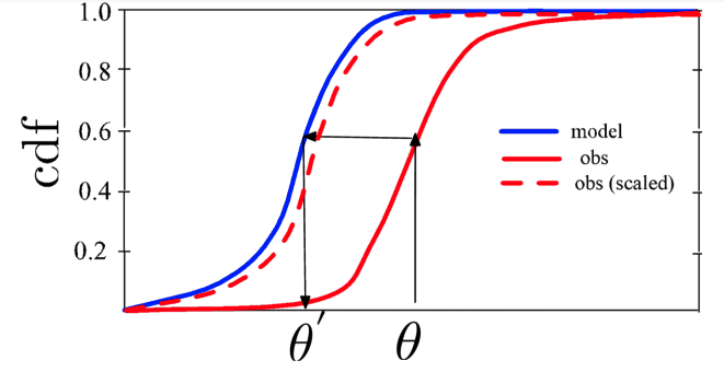

CDF generation and CDF-based scaling are performed separately for each grid point. CDF-based scaling corrects all moments of the distribution regardless of its shape and requires enough sampling density to derive these scaling parameters. By comparison, normal deviate-based scaling corrects the first and second moments (e.g., the mean and variance).

For more information on this topic:

Reichle, R. H., and Koster, R. D. (2004), Bias reduction in short records of satellite soil moisture, Geophys. Res. Lett., 31, L19501, doi:10.1029/2004GL020938.

Download Input and Target Files

The tar file for this step is approximately 384KB compressed and 803KB unpacked. Ensure that you have enough storage available before downloading testcase files.

% curl -O https://portal.nccs.nasa.gov/lisdata_pub/Tutorials/Web_Version/testcase4_ldt_lsmcdf_2023.tar.gz
% tar -xzf testcase4_ldt_lsmcdf_2023.tar.gz -C .

The following files and directories were added to your common working directory $WORKING_DIR:

DA_proc_LSM/

A directory containing the files below

ldt.config.noah36_cdf

The LDT config file for this step

target_ldtlog.0000

The target LDT log file

target_cdf_noah36_domain.nc

The target LDT-generated Noah LSM domain file

target_cdf_noah36.nc

The target LDT-generated Noah LSM CDF file

noah36_cdf.xdf

GrADS description file for viewing *cdf_noah36.nc output and target files

plot_noah36_cdf.gs

GrADS script that plots an X-Y plot of *cdf_noah36.nc output and target files

The LDT Configuration File

Review the contents of DA_proc_LSM/ldt.config.noah36_cdf to view the configuration settings used for this step:

LDT running mode: "DA preprocessing" (1)
...
DA preprocessing method:            "CDF generation"
DA observation source:              "LIS LSM soil moisture"
Name of the preprocessed DA file:   "cdf_noah36" (2)
Apply anomaly correction to obs:    0
Temporal resolution of CDFs:        "yearly"
Number of bins to use in the CDF:   100
Observation count threshold:        30
Temporal averaging interval:        "1da"
Apply external mask:                0
External mask director:             none
...
LIS soil moisture output model name:        "Noah.3.6"
LIS soil moisture output directory:         ../OL_OUTPUT/
LIS soil moisture output format:            "netcdf"
LIS soil moisture output methodology:       "2d gridspace"
LIS soil moisture output naming style:      "3 level hierarchy"
LIS soil moisture output nest index:        1
LIS soil moisture output map projection:    "latlon"
LIS soil moisture domain lower left lat:    34.375 (3)
LIS soil moisture domain upper right lat:   39.625
LIS soil moisture domain lower left lon:    -102.875
LIS soil moisture domain upper right lon:   -96.125
LIS soil moisture domain resolution (dx):   0.25
LIS soil moisture domain resolution (dy):   0.25

1	The "DA preprocessing" mode is used to generate the observation domain and scaling parameters.
2	A successful run will generate a domain file (i.e., `cdf_noah36_domain.nc`) and a LSM CDF file (e.g., `cdf_noah36.nc`).
3	The LDT run domain should reflect the intended observation grid (projection and resolution). Note that this can differ from the model resolution and projection.

Run LDT - DA Preprocessing Step

You’re now ready to run LDT:

Copy your compiled LDT executable into $WORKING_DIR/DA_proc_LSM
Run the LDT executable using the provided ldt.config.noah36_cdf file:

% ./LDT ldt.config.noah36_cdf

% tail ldtlog.0000
...
 --------------------------------
  Finished LDT run
 --------------------------------

LDT Output Files

During this run LDT produced a domain file, cdf_noah36_domain.nc, and a LSM CDF file, cdf_noah36.nc in the DA_proc_LSM directory. If GrADS is installed, use the provided GrADS descriptor files to plot the output shown below.

% grads -lc "plot_noah36_cdf.gs"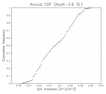

Step 5: Generate Observations CDF-based Files (LDT)

Overview

In this step you will use LDT to generate CDF files from the satellite-based soil moisture (SM) observations collected by NASA’s Soil Moisture Active Passive (SMAP) mission. The observation based CDF files generated in this step will be used along with the model CDF files created in Step 4 for the data assimilation run in Step 6.

Download Input and Target Files

The tar file for this step is approximately 4.6GB compressed and 9.1GB unpacked. Ensure that you have enough storage available before downloading testcase files.

% curl -O https://portal.nccs.nasa.gov/lisdata_pub/Tutorials/Web_Version/testcase5_ldt_obscdf_2023.tar.gz
% tar -xzf testcase5_ldt_obscdf_2023.tar.gz -C .

The following files and directories were added to your common working directory $WORKING_DIR:

RS_DATA.tgz

A tar file containing sample SMAP soil moisture observations

DA_proc_SMAP/

A directory containing the files below

ldt.config.smapobs_cdf

The LDT config file for this step

target_ldtlog.0000

The target LDT log file

target_cdf_smapobs_domain.nc

The target LDT-generated Noah LSM domain file

target_cdf_smapobs.nc

The target LDT-generated Noah LSM CDF file

The file RS_DATA.tgz should have been recursively unpacked as subdirectory RS_DATA within your $WORKING_DIR. If it was not, run the following command:

% tar -xzf RS_DATA.tgz -C .

The new directory, RS_DATA, contains sample soil moisture observations from the SMAP L3 Radiometer Global Daily 36 km EASE-Grid Soil Moisture data product.

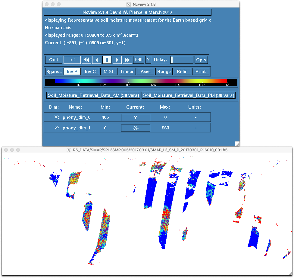
SMAP SPL3SMP.005 dataset description:

This Level-3 (L3) soil moisture product provides a composite of daily estimates of global land surface conditions retrieved by the Soil Moisture Active Passive (SMAP) passive microwave radiometer. SMAP L-band soil moisture data are resampled to a global, cylindrical 36 km Equal-Area Scalable Earth Grid, Version 2.0 (EASE-Grid 2.0).

Use ncview to view the data for 3/1/2017.

% ncview RS_DATA/SMAP/SPL3SMP.005/2017.03.01/SMAP_L3_SM_P_20170301_R16010_001.h5

When ncview opens, click and hold on one of the subdataset buttons under the color bar (e.g., Soil_Moisture_Retrieval_Data_AM (36 vars)) to open the list of variables. Release the mouse button on the variable you would like to plot (e.g., soil_moisture).

Due to the way the data is formatted, the plot will appear upside down. Click on the Inv P button in the main ncview window to invert the plot.

The LDT Configuration File

Review the contents of DA_proc_SMAP/ldt.config.smapobs_cdf to view the configuration settings used for this step:

LDT running mode: "DA preprocessing" (1)
...
DA preprocessing method:            "CDF generation"
DA observation source:              "NASA SMAP soil moisture"
Name of the preprocessed DA file:   "./cdf_smapobs" (2)
Apply anomaly correction to obs:    0
Temporal resolution of CDFs:        "yearly" (3)
Number of bins to use in the CDF:   100
Observation count threshold:        30
Temporal averaging interval:        "1da"(4)
Apply external mask:                0
External mask director:             none
...
NASA SMAP soil moisture observation directory: ../RS_DATA/SMAP/SPL3SMP.005  (5)
NASA SMAP soil moisture data designation:      SPL3SMP (6)
NASA SMAP search radius for openwater proximity detection: 3 (7)
SMAP(NASA) soil moisture Composite Release ID (e.g., R16): R16 (8)

1	DA preprocessing mode is used to generate the observation domain and scaling parameters.
2	Prefix of output files (e.g., `cdf_smapobs_domain.nc`).
3	Temporal resolution of resultant CDF. Specifies whether to generate lumped (i.e., considering all years and all seasons) CDFs or to stratify CDFs for each calendar month.
4	Averaging interval used while computing the CDF. In this case, one day.
5	Relative path to the directory containing SMAP observation data.
6	Specifies which SMAP data product is being used.
7	Specifies the radius in which LDT searches to detect open water. Then removes all pixels within the radius in the CDF calculations.
8	Specifies the release ID of the SMAP dataset.

See the LDT Users' Guide for more information about configuration settings.

Run LDT - DA Preprocessing Step

You’re now ready to run LDT:

Copy your compiled LDT executable into $WORKING_DIR/DA_proc_SMAP
Run the LDT executable using the provided ldt.config.smapobs_cdf file:

% ./LDT ldt.config.smapobs_cdf

% tail ldtlog.0000
...
 --------------------------------
  Finished LDT run
 --------------------------------

The run created two new files:

cdf_smapobs.nc
cdf_smapobs_domain.nc

Use ncview to plot the SoilMoist_domain variable contained in cdf_smapobs_domain.nc:

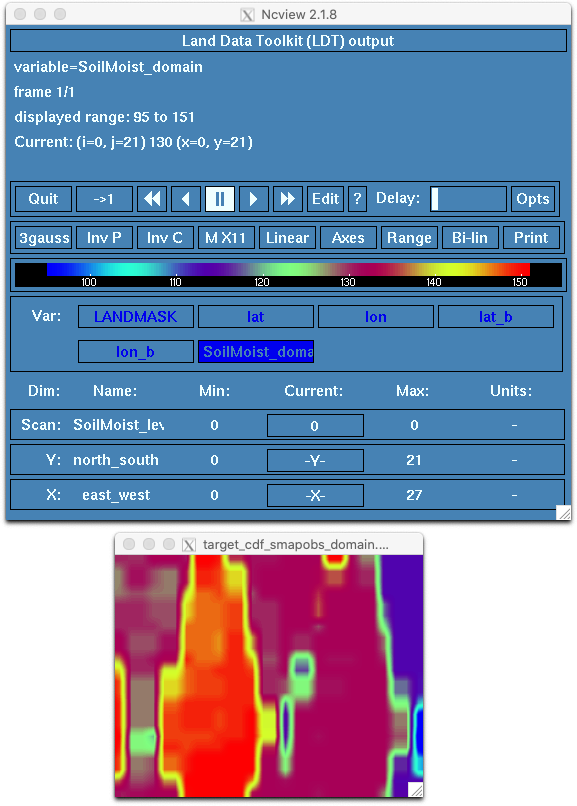
Use nccmp to directly compare the contents of cdf_smapobs_domain.nc with the provided target. They should be identical.

% nccmp -dsf cdf_smapobs_domain.nc target_cdf_smapobs_domain.nc
Files "cdf_smapobs_domain.nc" and "target_cdf_smapobs_domain.nc" are identical.

Wrap Up

You now have all of the files needed to perform the data assimilation run.

Step 6: LSM Data Assimilation (DA) Experiment (LIS)

Overview

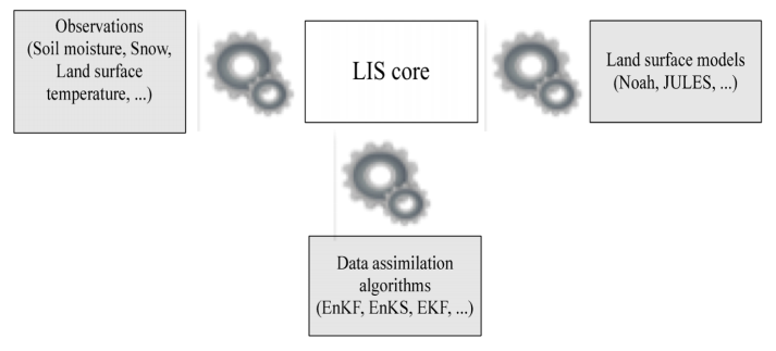
The Data Assimilation (DA) subsystem in LIS is primarily used for state estimation (i.e., correction of model states based on observations) and supports the interoperable use of multiple land surface models, algorithms, and observational data sources. The DA subsystem also provides support for concurrent data assimilation, forward models, radiance assimilation, and observation operators employing advanced data fusion methods (i.e., deep learning). Advanced data assimilation algorithms such as Ensemble Kalman Filter (EnKF) and Ensemble Kalman Smoother (EnKS) are available.

For more information:

Kumar, S. V., R. H. Reichle, C. D. Peters-Lidard, R. D. Koster, X. Zhan, W. T. Crow, J. B. Eylander, and P. R. Houser, 2008: A Land Surface Data Assimilation Framework using the Land Information System: Description and Applications, Adv. Wat. Res., 31, 1419-1432, doi:10.1016/j.advwatres.2008.01.013.

The DA subsystem outputs a number of diagnostics including:

DA innovations, normalized innovations, and ensemble spread
Processed/bias-corrected/quality-controlled (QC’d) observational data

The Land Verification Toolkit (LVT) handles automated processing of these outputs.

Example DA output: variance of normalized innovations

Download Input and Target Files

The tar file for this step is approximately 80MB compressed and 327MB unpacked. Ensure that you have enough storage available before downloading testcase files.

% curl -O https://portal.nccs.nasa.gov/lisdata_pub/Tutorials/Web_Version/testcase6_lis_da_2023.tar.gz
% tar -xzf testcase6_lis_da_2023.tar.gz -C .

The following directories and files were added to your common working directory $WORKING_DIR:

DA_INPUT/

Contains the perturbation files used in the DA run

lis.config_noah36_smapda

The LIS config file for this step

target_SMAPDA_OUTPUT/

Contains the target DA output generated by LIS

target_log/lislog_smapda.0000

The target LIS log file

target_da.xdf & test_da.xdf

GrADS description files to view the output

This step relies on files downloaded or generated in the previous steps. In addition to the files just downloaded, ensure the following directories are present in $WORKING_DIR:

DA_ensrst/

Ensemble restart files generated in Step 3

DA_proc_LSM/

LSM-based CDF files generated in Step 4

DA_proc_SMAP/

Observations-based CDF files generated in Step 5

RS_DATA/

Observation data files downloaded in Step 5

INPUT/

NLDAS2 forcing and Noah model files downloaded in Step 2

The LIS Configuration File

Review the contents of lis.config_noah36_smapda to view the configuration settings used for the DA run:

Restart options:

...
Start mode:                                restart (1)
...
Number of ensembles per tile:              12 (2)
...
Noah.3.6 restart file:                    ./DA_ensrst/LIS_EnRST_NOAH36_201801010000.d01.nc (3)
...

1	Select "restart" mode to use a restart file (as opposed to "coldstart" mode).
2	# of ensemble members to use (matches ensemble restart file).
3	Filepath of the 12 member ensemble restart file generated in Step 3.

Data assimilation options:

...
Number of data assimilation instances:               1

Data assimilation algorithm:                         "EnKF"
Data assimilation set:                               "SMAP(NASA) soil moisture"
Number of state variables:                           4
Data assimilation use a trained forward model:       0
Data assimilation trained forward model output file: none
Data assimilation exclude analysis increments:       0
Data assimilation output interval for diagnostics:  "1da"
Data assimilation number of observation types:       1
Data assimilation output ensemble spread:            1
Data assimilation output processed observations:     1
Data assimilation output innovations:                1
...

Scaling strategy options:

...
Data assimilation scaling strategy:         "CDF matching"
Data assimilation observation domain file:  ./lis_input.nldas.noah36.d01.nc

Bias estimation algorithm:                  "none"
Bias estimation attributes file:            "none"
Bias estimation restart output frequency:
Bias estimation start mode:
Bias estimation restart file:
...

Perturbation options:

...
Perturbations start mode:                 "coldstart"
Perturbations restart output interval:    "1mo"
Perturbations restart filename:           "none"
Apply perturbation bias correction:       0
...
Forcing perturbation algorithm:           "GMAO scheme" (1)
Forcing perturbation frequency:           "1hr"
Forcing attributes file:                  ./DA_INPUT/forcing_attribs.txt
Forcing perturbation attributes file:     ./DA_INPUT/forcing_pert_attribs.txt

State perturbation algorithm:             "GMAO scheme" (2)
State perturbation frequency:             "6hr"
State attributes file:                    ./DA_INPUT/noah_sm_attribs.txt
State perturbation attributes file:       ./DA_INPUT/noah_sm_pertattribs.txt

Observation perturbation algorithm:       "GMAO scheme" (3)
Observation perturbation frequency:       "6hr"
Observation attributes file:              ./DA_INPUT/smap_attribs.txt
Observation perturbation attributes file: ./DA_INPUT/smap_pertattribs.txt

1	Forcing perturbation options
2	State perturbation options
3	Observation perturbation options

Observation data options:

SMAP(NASA) soil moisture data designation:       SPL3SMP
SMAP(NASA) soil moisture data directory:        ./RS_DATA/SMAP/SPL3SMP.005
SMAP(NASA) soil moisture use scaled standard deviation model: 0
SMAP(NASA) soil moisture apply SMAP QC flags:                 1
SMAP(NASA) model CDF file:              ./DA_proc_LSM/cdf_noah36.nc
SMAP(NASA) observation CDF file:        ./DA_proc_SMAP/cdf_smapobs.nc
SMAP(NASA) soil moisture number of bins in the CDF:          100
SMAP(NASA) CDF read option: 0
SMAP(NASA) soil moisture use scaled standard deviation model: 0
SMAP(NASA) soil moisture Composite Release ID: R16

See the LIS Users' Guide for more information about configuration settings.

The Perturbation Configuration Files

Forcing Perturbations

Forcing variables and perturbation settings are defined in the files named forcing_attribs.txt and forcing_pert_attribs.txt, respectively. The paths to these files are set in the LIS configuration file (see Forcing perturbation options annotation above).

forcing_attribs.txt specifies the variables and their ranges:

#nfields
4
#varmin  varmax
Incident Shortwave Radiation Level 001
0.       1300.
Incident Longwave Radiation Level 001
-50.     800.
Rainfall Rate Level 001
0.0      0.001
Near Surface Air Temperature Level 001
220.0    330.0

For each variable listed in the snippet above, the name is given followed by the min and max values.

forcing_pert_attribs.txt specifies perturbation settings:

#ptype   std    std_max   zeromean  tcorr  xcorr ycorr ccorr
Incident Shortwave Radiation Level 001
1        0.20   2.5       1         86400  0     0     1.0  -0.3 -0.5  0.3
Incident Longwave Radiation Level 001
0        30.0   2.5       1         86400  0     0    -0.3   1.0  0.5  0.6
Rainfall Rate Level 001
1        0.50   2.5       1         86400  0     0    -0.5   0.5  1.0  -0.1
Near Surface Air Temperature Level 001
0        0.5    2.5       1         86400  0     0     0.3   0.6  -0.1  1.0

In the snippet above, the column headings represent:

ptype: Perturbation type; additive (0) or multiplicative (1)
std: Standard deviation of perturbations
std_max: Maximum allowed normalized perturbation relative to N(0, 1)
zeromean: Enforce zero mean across the ensemble; off (0) or on (1)
tcorr: Temporal correlation scale (in seconds) used in the AR(1) model
xcorr & ycorr: Spatial correlation scale (deg)
ccorr: Cross-correlations with other variables

State Perturbations

State variables and perturbation settings are defined in the files named noah_sm_attribs.txt and noah_sm_pertattribs.txt, respectively. The paths to these files are set in the LIS configuration file (see State perturbation options annotation above).

noah_sm_attribs.txt specifies perturbation settings:

#nfields
4
#varmin  varmax
Soil Moisture Layer 1
 0.01    0.55
Soil Moisture Layer 2
 0.01    0.55
Soil Moisture Layer 3
 0.01    0.55
Soil Moisture Layer 4
 0.01    0.55

noah_sm_pertattribs.txt specifies the variables and their ranges:

#perttype  std    std_max   zeromean  tcorr    xcorr ycorr ccorr
Soil Moisture Layer 1
  0        0.02   0.1       1          10800   0     0     1.0 0.0 0.0 0.0
Soil Moisture Layer 2
  0        0.00   0.1       1          10800   0     0     0.0 1.0 0.0 0.0
Soil Moisture Layer 3
  0        0.00   0.1       1          10800   0     0     0.0 0.0 1.0 0.0
Soil Moisture Layer 4
  0        0.00   0.1       1          10800   0     0     0.0 0.0 0.0 1.0

Observation Perturbations

Observation variables and perturbation settings are defined in the files named smap_attribs.txt and smap_pertattribs.txt, respectively. The paths to these files are set in the LIS configuration file (see Observation perturbation options annotation above).

smap_attribs.txt specifies perturbation settings:

#nfields
1
#varmin  varmax
SMOPS soil moisture
 0.01    1.0

smap_pertattribs.txt specifies the variables and their ranges:

#perttype std  std_max  zeromean  tcorr  xcorr ycorr ccorr
SMOPS soil moisture
 0        0.04 2.5      1         43200  0     0     1.0

Run LIS - SMAP DA Experiment

You’re now ready to run LIS to perform the SMAP DA experiment. From $WORKING_DIR, run the LIS executable with the config file for this step:

./LIS -f lis.config_noah36_smapda

Using one processor, as we are here, the run will take approximately 30 minutes to complete. If the run fails, troubleshoot the issue by reviewing any errors printed to the terminal and by viewing the contents of log/lislog_smapda.0000. If no errors print to the terminal, verify that the run completed successfully by checking for the following confirmation at the end of log/lislog_smapda.0000:

% tail lislog_smapda.0000
...
LIS Run completed.

View the output of the run using GrADS, ncview, Matlab, or other software. Compare the output generated by this run with the output of the Open-Loop case from Step 2.

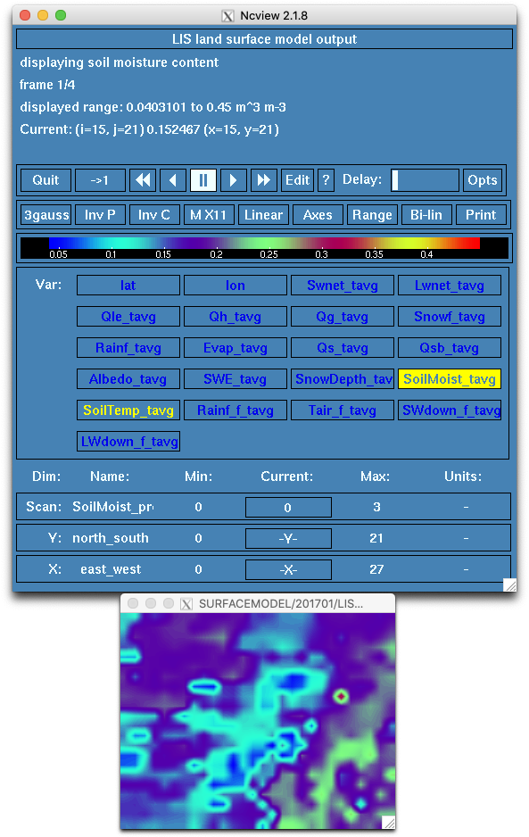
SoilMoist_tavg variable in LIS_HIST_201701010600.d01.nc

Wrap Up

You have completed the SMAP Data Assimilation Experiment. In Step 7, you will use the Land Verification Toolkit (LVT) to process the output of the OL and DA runs.

Step 7: Comparison of OL and DA Experiments (LVT)

Overview

In this step, you will use the Land Verification Toolkit (LVT) to compare the output generated in the open-loop (Step 2) and data assimilation (Step 6) experiments. Since LVT is a verification and validation software, you will need to plot the output using Python, Matlab, GrADS, etc. LVT offers a range of features and configuration settings so we strongly encourage users to review the LVT Users' Guide.

Download Input and Target Files

The tar file for this step is approximately 481KB compressed and 7.2MB unpacked. Ensure that you have enough storage available before downloading testcase files.

% curl -O https://portal.nccs.nasa.gov/lisdata_pub/Tutorials/Web_Version/testcase7_lvt_expcomp_2023.tar.gz
% tar -xzf testcase7_lvt_expcomp_2023.tar.gz -C .

The following files and directories were added to your common working directory $WORKING_DIR:

lvt.config.ol.da

The LVT config file for the OL and DA runs

lvt.config_smapDAobs

The LVT config file for the SMAP observations used in the DA run

METRICS.TBL

A text file that defines the statistical metric options used by LVT

TS_LOCATIONS.TXT

A text file that specifies the points or regions in the domain where ASCII time series data are to be derived

target_STATS.ol.da/

A directory containing the target LVT output for the OL and DA runs

target_STATS.smapDAobs/

A directory containing the target LVT output for the SMAP DA obs run

target_log/

A directory containing target log files

target_fig/

A directory containing target figures

plot_TS.m

A Matlab script to generate plots of the output

plot_noah36_smapda_littlewashita.plt plot_noah36_smapda_fortcobb.plt

gnuplot scripts to generate plots of the output

The LVT Configuration Files

Review the two LVT configuration files for this step.

lvt.config.ol.da:

#Overall driver options
LVT running mode:                       "Data intercomparison"
Map projection of the LVT analysis:     latlon
LVT output format:                      netcdf
LVT output methodology:                 "2d gridspace"

Analysis data sources:               "LIS output"  "LIS output"
...

#     Datastream 1             |            Datastream 2
LVT datastream attributes table::
SoilMoist  1 1  m3/m3   - 1 4     SoilMoist  1 1  m3/m3    - 1 4
RootMoist  1 1  m3/m3   - 1 1     RootMoist  1  1 m3/m3    - 1 1
...

lvt.config.smapDAobs:

#Overall driver options
LVT running mode:                       "Data intercomparison"
Map projection of the LVT analysis:     latlon
LVT output format:                      netcdf
LVT output methodology:                 "2d gridspace"

Analysis data sources:                  "LIS DAOBS"  "none"
...

## DATA STREAM INPUTS ....

#Observation
LIS DAOBS output directory:  ./SMAPDA_OUTPUT/DAOBS
LIS DAOBS domain file:       ./lis_input.nldas.noah36.d01.nc
LIS DAOBS instance index:     1
LIS DAOBS use scaled obs:     1
LIS DAOBS output interval:    "15mn"
LIS DAOBS observation type:   "soil moisture"
...

Running LVT

First, run LVT to process the OL vs. DA soil moisture output:

% ./LVT lvt.config.ol.da

If the run fails, troubleshoot the issue by reviewing any errors printed to the terminal and by viewing the contents of any log files present (e.g., lvtlog*.0000). Otherwise, verify that the run completed successfully by checking for the confirmation message at the end of lvtlog_ol_da.0000:

% tail lvtlog_ol_da.0000
...
[INFO] Finished LVT analysis
 [INFO] --------------------------------------

The output generated by this run can be found in the STATS.ol.da directory and should include point data for "Fort Cobb" and "Little Washita", locations specified in the TS_LOCATIONS.txt file. Compare these files with the target output in target_STATS.ol.da using nccmp to compare the NetCDF files and diff to compare the .dat files.

Next, run LVT to process the SMAP DA observations so it can be easily compared with our model output:

% ./LVT lvt.config.smapDAobs

% tail lvtlog.smapDAobs.0000
...
[INFO] Finished LVT analysis
 [INFO] --------------------------------------

The output generated by this run can be found in the STATS.smapDAobs directory and should include point data for "Fort Cobb" and "Little Washita", locations specified in the TS_LOCATIONS.TXT file. Again, compare these files with the target output in target_STATS.smapDAobs using nccmp to compare the NetCDF files and diff to compare the .dat files.

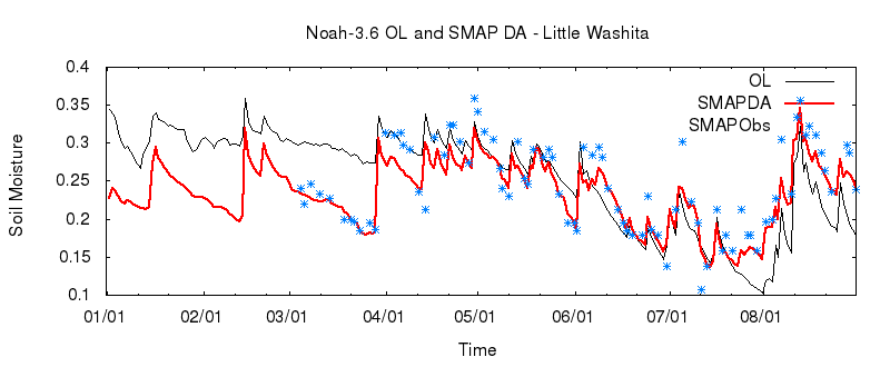
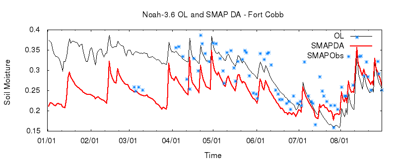
Plot the Results

We can now compare the results of our OL and DA runs with the observations we assimilated. Sample scripts to generate plots with gnuplot (plot_noah36_smapda_*.plt) and Matlab (plot_TS.m) are included among the input files.

The gnuplot and Matlab scrips mentioned above expect the existence of a $WORKING_DIR/fig directory as a location to save figures. The scripts will not automatically make this directory. Therefore, prior to running these scripts, you must manually create a $WORKING_DIR/fig directory.

`gnuplot` Plots

Matlab Plots

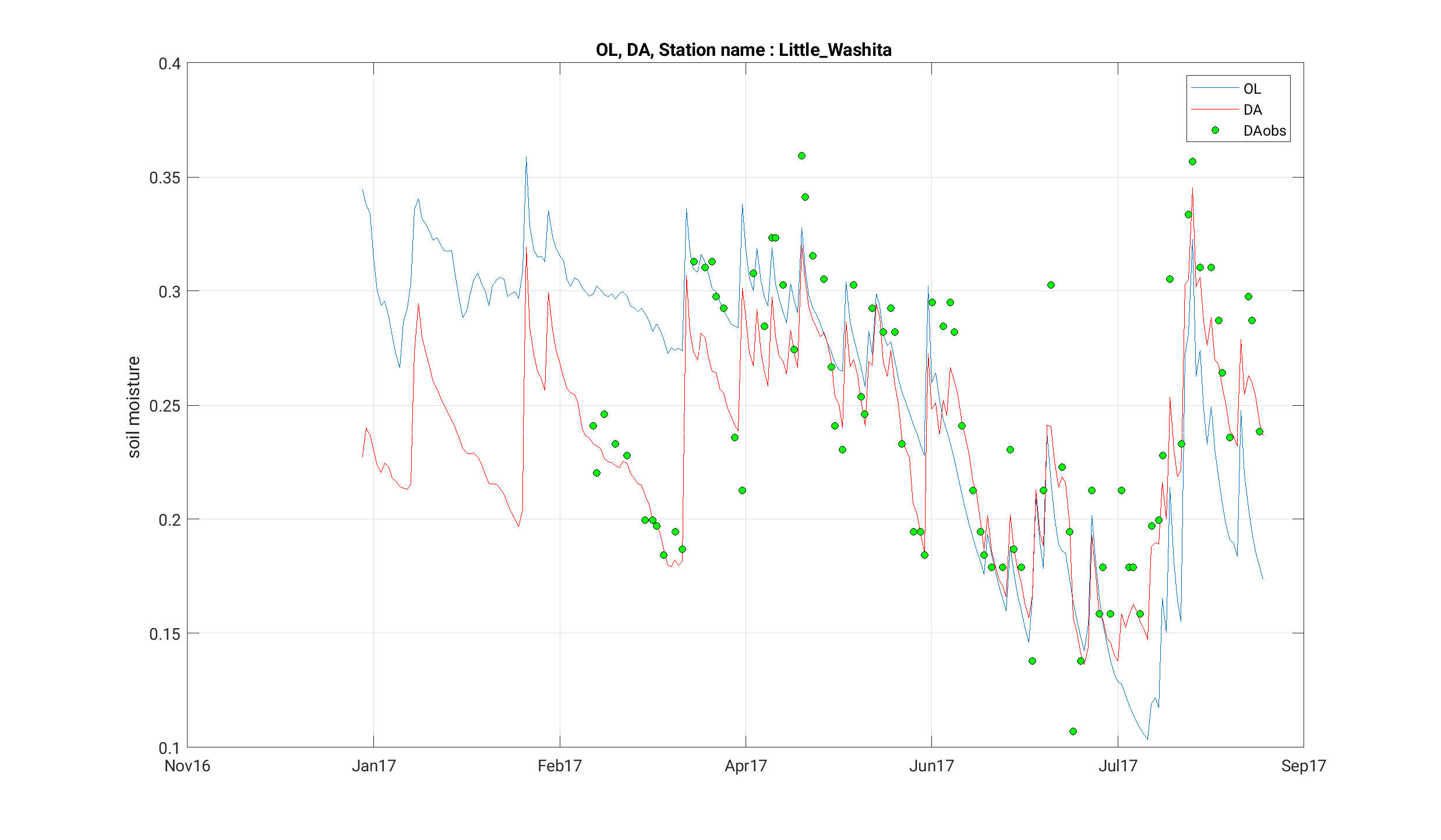
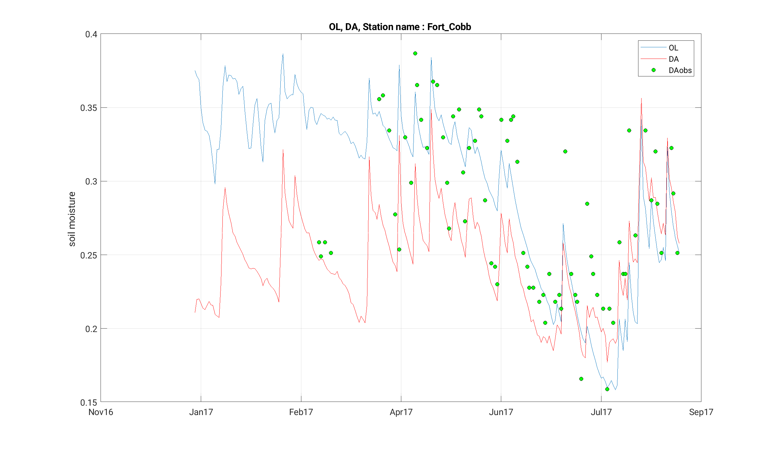
Wrap Up

You have now completed the end-to-end public testcase for NASA’s Land Information System.

LIS Public Testcase Walkthrough

Introduction

The Testcase Event: Snow Blankets the Southern Great Plains

Setup

Create a working directory

Clone the LISF Repository

Configure and Compile the LISF Components

Step 1: LSM Parameter Processing Run (LDT)

Overview

Steps to Running LDT

Download Input and Target Files

The LDT Configuration File

Noah Land Surface Model Parameters

Testcase Domain

Run LDT - The Parameter Processing Step

LDT Output Files

The LIS Parameter File

Compare the Output

Wrap-up

Step 2: LSM "Open-loop" (OL) Experiment (LIS)

Overview

Steps to Running LIS

Download Input and Target Files

Download the Meteorological Forcing Dataset

The LIS Configuration File

Run LIS - The "Open-Loop" (OL) Step

LIS Output Files

Wrap-up

Step 3: Ensemble Restart File Generation (LDT)

Overview

Download Input and Target Files

The LDT Configuration File

Run LDT - Generate Ensemble Restart File

LDT Output Files

Step 4: Generate LSM OL Cumulative Density Function-based Files (LDT)

Overview

Download Input and Target Files

The LDT Configuration File

Run LDT - DA Preprocessing Step

LDT Output Files

Step 5: Generate Observations CDF-based Files (LDT)

Overview

Download Input and Target Files

The LDT Configuration File

Run LDT - DA Preprocessing Step

Wrap Up

Step 6: LSM Data Assimilation (DA) Experiment (LIS)

Overview

Download Input and Target Files

The LIS Configuration File

The Perturbation Configuration Files

Forcing Perturbations

State Perturbations

Observation Perturbations

Run LIS - SMAP DA Experiment

Wrap Up

Step 7: Comparison of OL and DA Experiments (LVT)

Overview

Download Input and Target Files

The LVT Configuration Files

Running LVT

Plot the Results

gnuplot Plots

Matlab Plots

Wrap Up

`gnuplot` Plots